In the modern machine learning landscape, we've all become used to a certain form of answer from our models. When we train a neural network to help us with a regression problem, a smashing success is a model that gives us outputs that seem reasonable and consistent with the data we've seen before. However, an important piece of information that is often overlooked is the confidence of our model's prediction. When a neural network hands you a predicted function value for some input, you have a guess of where the function will be at a certain point but you can't say much in terms of how likely you think it is that that value will actually occur there, or how far from that value we might be nine times out of ten.
It doesn't take a lot of imagination to come up with a situation in which it is just as important to have a prediction of a function at some point in time as it is to have a confidence interval around that prediction. The reason neural networks leave us high and dry on this front is that a trained model is deterministic by design. After a neural network is fit to our training data, it is simply the function that resembles the most likely generator of the points we gave it.
The reason that these predictions can fail us is the simple fact that the most likely outcome is often not what ends up actually happening. Shifting to the language of probability, we can think of a regression function as a random variable drawn from a distribution. Because of the way that neural networks are built, when we set out to calculate a regression function for some training points we have, we are only able to make a single draw from the distribution of possible functions. If we were able to make many draws, or somehow preserve knowledge of the distribution that's giving us regression functions, suddenly the ability to get undercertainty measures on our predictions doesn't seem farfetched at all.
Gaussian processes are a tool that let us do exactly that, and below we'll walk through some simple examples that will give us an intuition for thinking about regression problems through the lens of probability distributions.
In order to talk about Gaussian processes, we'll start with the basics of what makes them "Gaussian" in the first place.
A good starting point is to consider a multivariate Gaussian:
This is a \(3\)-dimensional random variable and from our definition we're saying that each component \(f_i\), if consideredd on its own, is drawn from a single-variable Gaussian distribution with mean \(\mu_i\) and variance \(\sigma_i^2\). All we've done to put these three variables into \(F\) is form the vector \(\mu\) to describe the three components' means altogether, and because the components are dependent on each other (i.e., correlated) we create the matrix \(\Sigma\) with entries \(K_{ij} = K(t_i,t_j)\) to give the covariance of elements \(f_i\) and \(f_j\), defined by some covariance function \(K\). This function \(K\) can take many different forms, but right now all we need to know is that it gives us a measure of the relation between points.
One common simplifying assumption we'll make is that all of our variables \(f_i\) have a mean of zero. This isn't a very consequential choice to make, as we could always achieve this by shifting a variable to be centered at zero. For ease of notation, we'll rewrite our distribution of \(F\) as
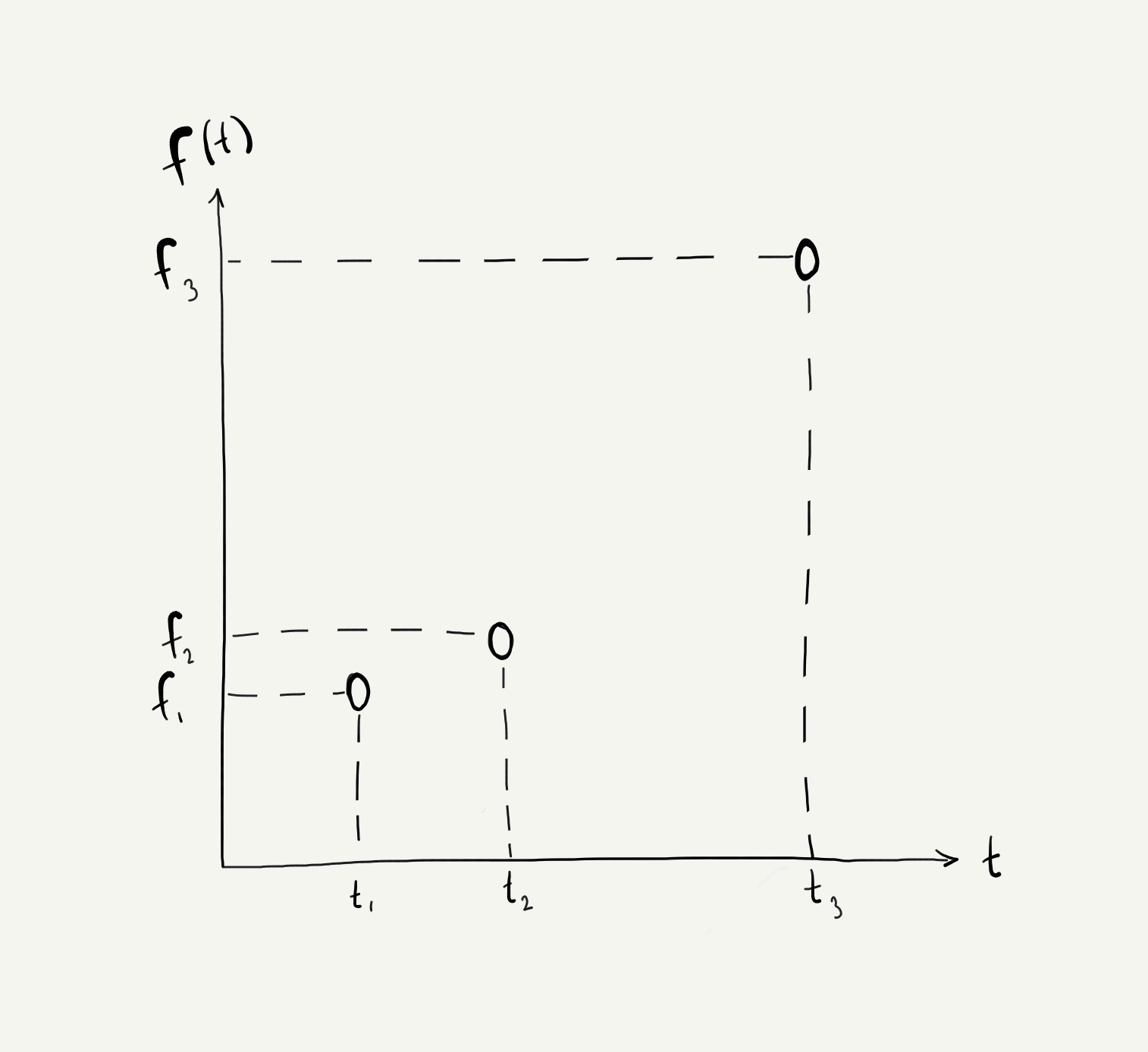
Now that we have our 3-dimensional variable \(F\), let's consider the world in which each component \(f_i\) occurred at a some time \(t_i\). It would make a lot of sense to place these variables on a plot like this:
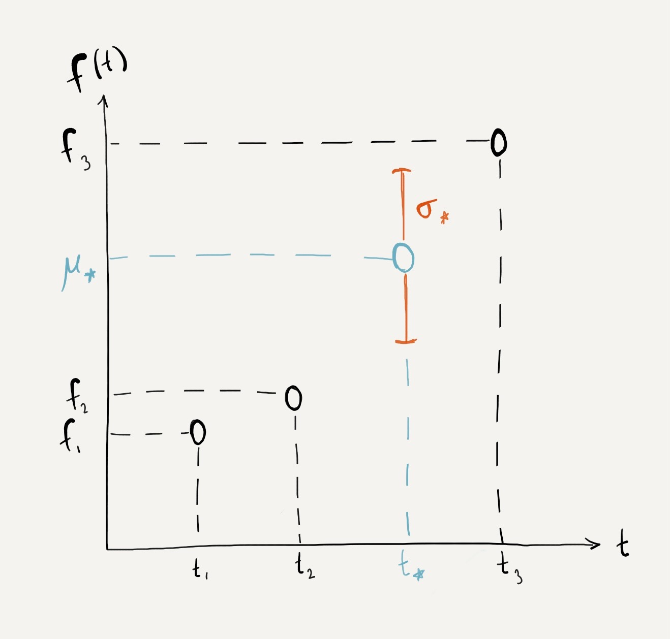
If we're setting out to fill in gaps in our data, we might want to try and estimate what kinds of \(f\) values occur between \(t_2\) and \(t_3\). So let's do this for a specific point \(t_*\) that we'll choose between \(t_2\) and \(t_3\), and see what we know about \(f_*\).
Using the definitions we've set up so far, we can say a few things about \(f_*\) right off the bat. First, because we're assuming it will be generated by the same process as the other points, we can say that it will come from a Gaussian distribution with zero mean and a variance given by our function \(K\).
Adding this value \(f_*\) into the our original 3-dimensional random variable \(F\), we have the new 4-dimensional random variable \(F^*\).
... and to tidy things up a we can group these terms to separate the known quantites from \(F\) from the unknown quantites from our predicted point \(f_*\) (and we'll define \(K_*\) to be the vector made up of the entries on the right side of the covariance matrix, \(K_{1*}, K_{2*}, K_{3*}\))
With our assumption that \(F^*\) is a multivariate Gaussian with \(f_*\) as a component, the distribution of \(f_*\) can be found as a conditional distribution of \(F^*\) using the Multivariate Gaussian Theorem (Bishop,Pattern Recognition and Machine Learning, Section 2.3.1) to get the mean and variance of our new point.
The proof of the Multivariate Gaussian Theorem isn't important for understanding this example, it is just a result of the conditional distributions of multivariate Gaussians. At this point, what we've just arrived at are the expected value and variance that we'll expect to see from our function at the new point \(t_*\)
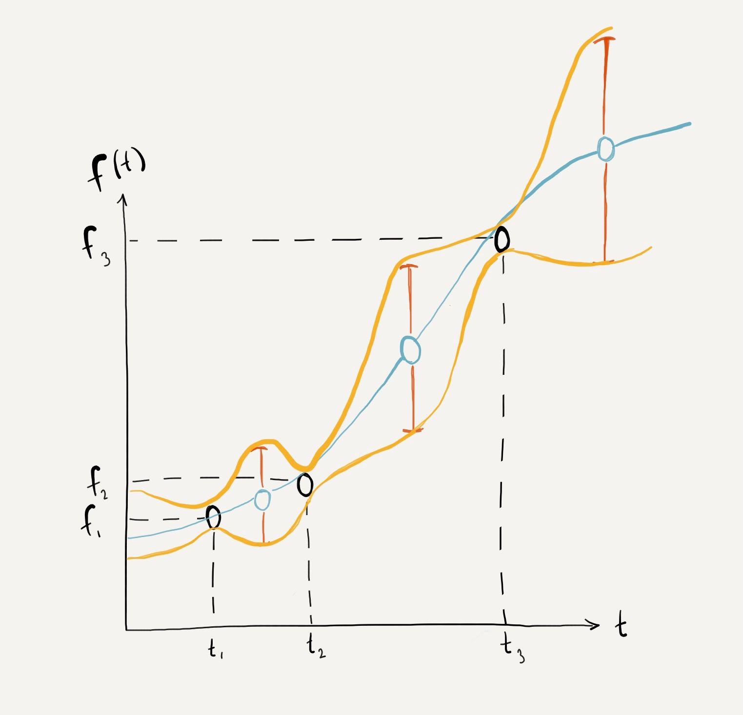
Tying this idea back to our notation from earlier, we can express our infinite-dimensional Gaussian random variable as
and we can replace our random variable with the equivalent function \(f(t)\), and name the distribution it comes from as a distribution that's defined by a mean function and a covariance function \(f(t) \sim GP(m(t), K(t, t'))\) This formulation brings us to the definition of a Gaussian process, as a distribution over functions. Just as a Gaussian distribution is defined by a mean and covariance, a Gaussian process is defined by a mean function and covariance function.
The formal definition of a Gaussian process is a collection of random variables, any finite number of which have a joint Gaussian distribution. (Williams and Rasmussen, 2005, p.13)
Now that we've gone through this example and arrived at our definition, we're starting to build an intuition for how you might be able to be able to start from a set of training points and then find a distribution that will allow us make many draws of possible regression functions. To drive home the idea that a Gaussian process is a distribution, here's the result of doing what we just did above in code.
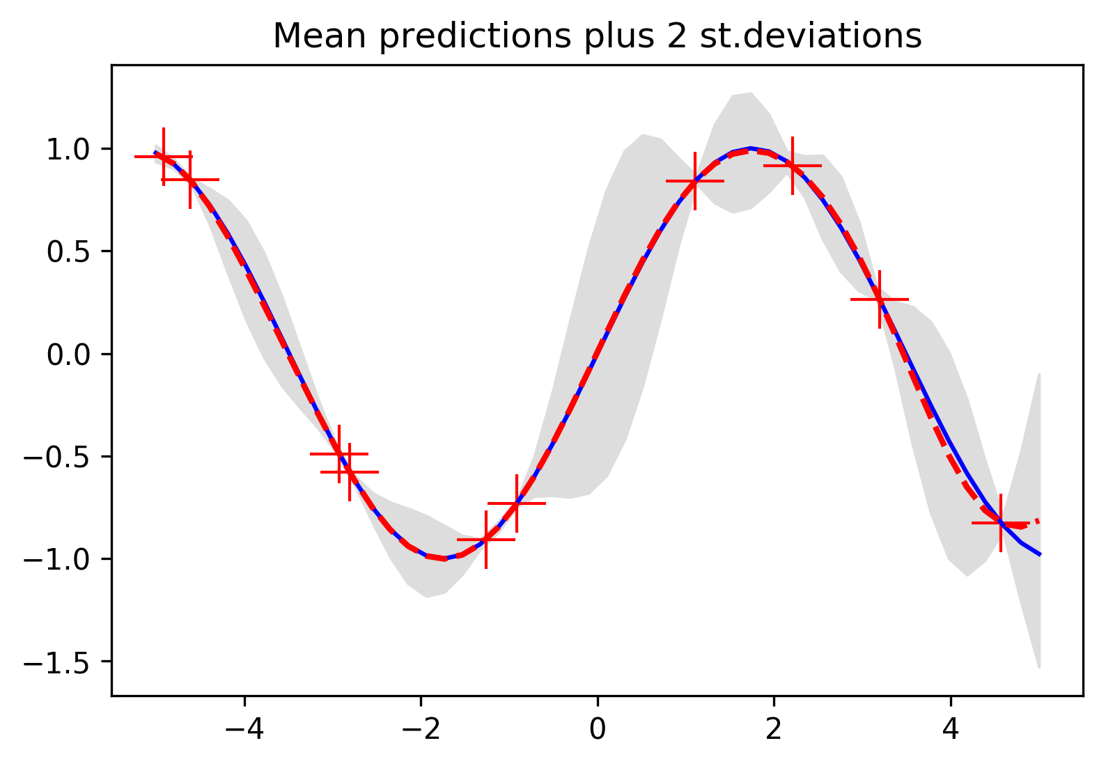
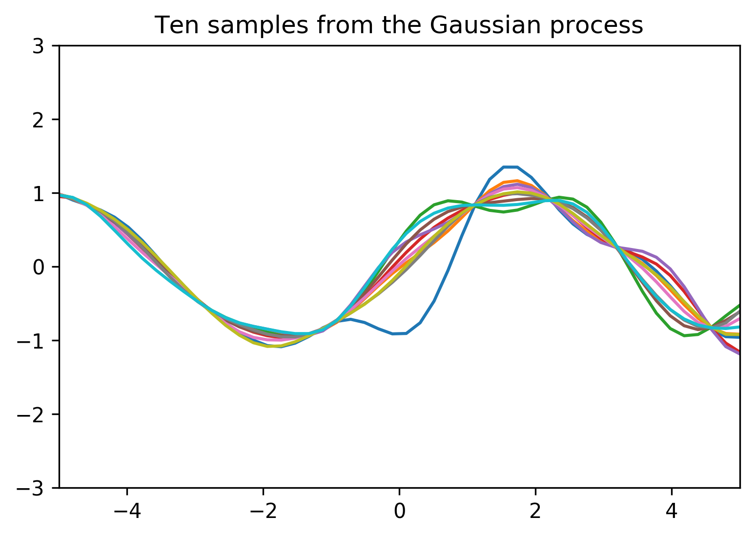
The top graph shows exactly the same result we reached when we interpolated to get confidence intervals of new possible points that our function might take on. These confidence intervals are shown for every possible value along the x-axis in grey, and they shade in the area that defines our Gaussian process. And because the Gaussian process is a distribution over functions, we can sample functions from it as much as we want, and ten such samples are shown in the second graph here. Most intuitively of all, each of these samples looks like something you might draw if you were given these training points asked to draw the regression function with a marker. Where there are points you know for sure, all of your guesses will pass through them, but whenever we have a big gap between points there are more possibilities for where the function might go in between.
So we've just seen how Gaussian processes move us into the world of distributions where we're able to have a continuously-defined idea of how uncertain our prediction is, but this isn't the only benefit to this appoach. A huge reason that Gaussian processes are a popular method of modeling is the fact that we can encode behavior that we want to see in our regression function with the careful choice of a covariance function. In our example we used a covariance function that very simply says that points that are closer in time should be more correllated. The actual function is the squared exponential kernel
This is a type of object called a \emph{kernel function}, and it's a member of a much larger family of different kernel functions that are very useful for describing different covariance patterns between points. The squared exponential kernel that we used is a very common one, mostly because it is a simple way to enforce smoothness across our function, but other choices of kernels can tell our regression function to anticipate different types of behavior that we might want it to model. For example, if we were modeling weather data that we knew was going to have a lot of periodicity in it, we could give our Gaussian process a periodic kernel like
Let's take a look at what our predictions might look like if we fit our points from before using this periodic kernel...
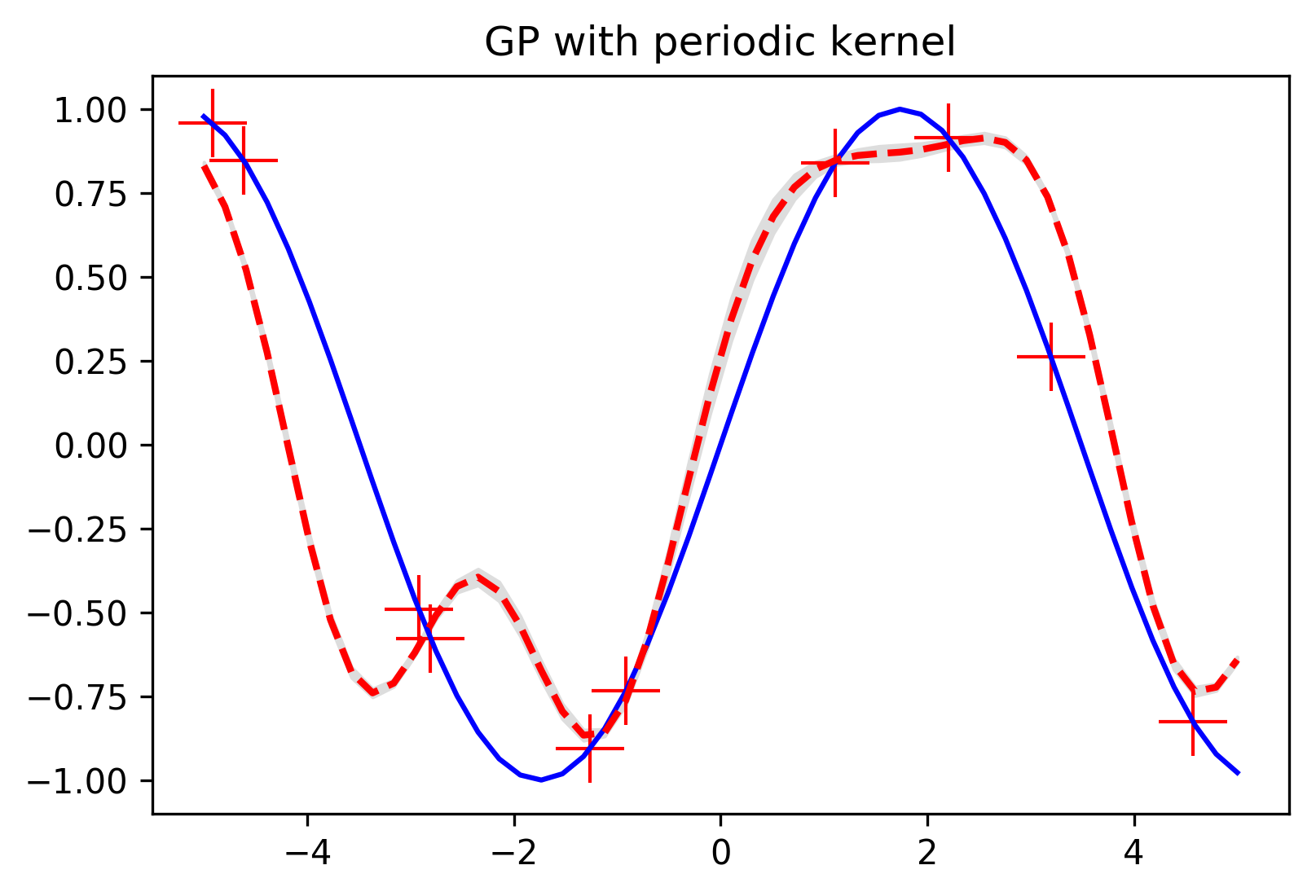
We can see the periodic kernel in action in the spaces between our training points where the Gaussian process is predicting periodic trends.
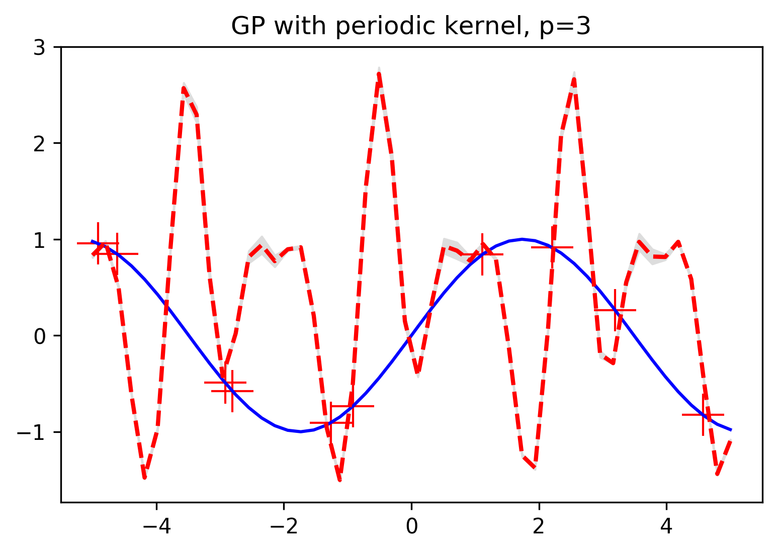
And of course in order to make full use of these kernel functions, we need to be able to tune any hyperparameters that might specify the scale of the trends we're imposing on our regression functions. For example, this periodic kernel has a parameter \(p\) which specifies the periodicity of the function. Here's an example of the prediction we get using a smaller value of \(p\) which will tell out Gaussian processes to expect much faster oscillation:
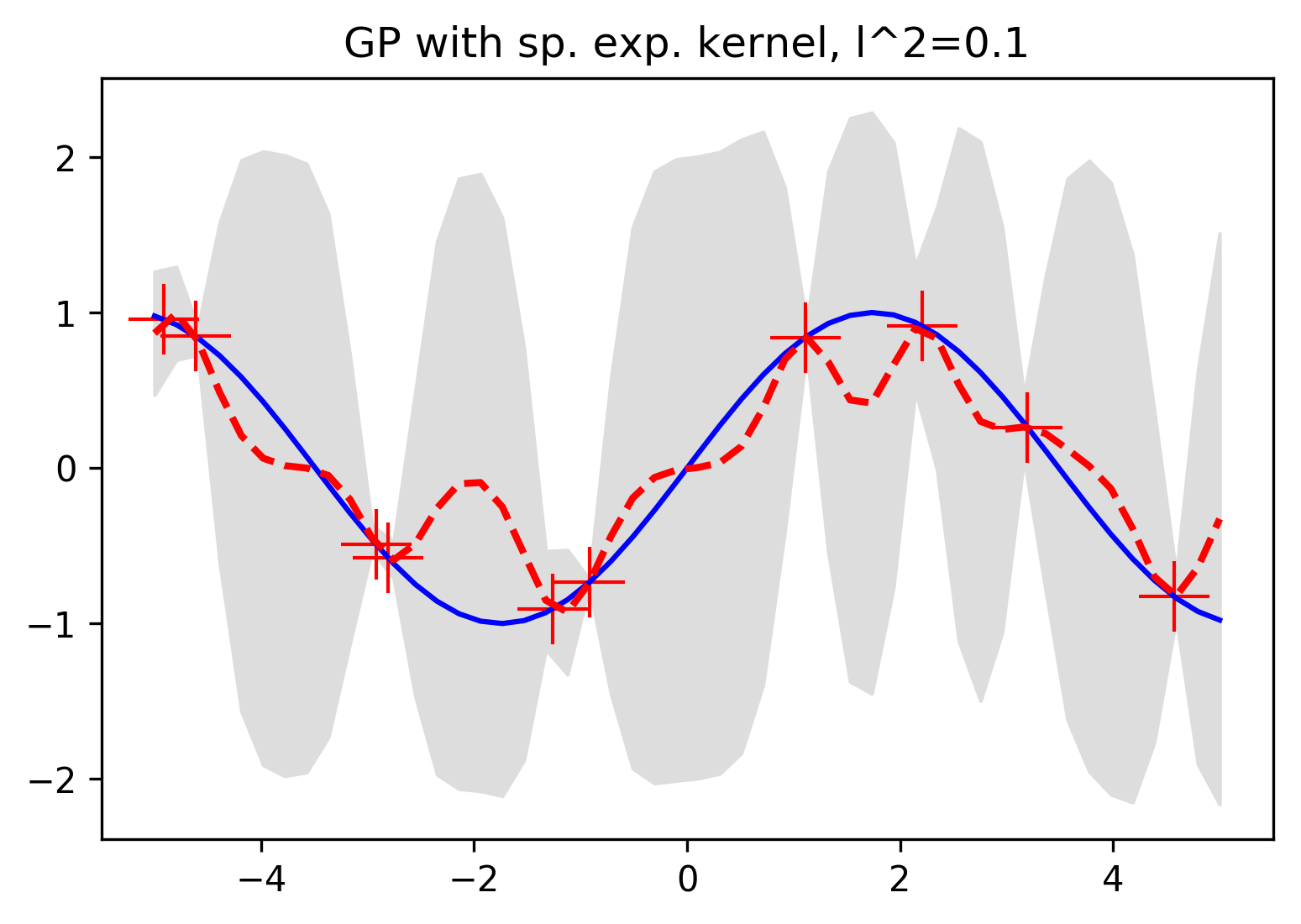
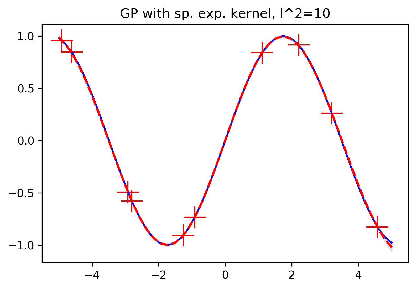
And taking a look back to the squared exponential kernel, here's what happens when we change the parameter \(l\), which specifies the length of the window in which training points will influence predictions. With a smaller value of \(l\), our prediction at a given point will only be influenced by very nearby training points, and with a large value we'll see training points influence observations much farther away.
Now that we've built up our definition of Gaussian processes and seen a few ways in which they can give us a lot of extra information and control over our model, we can reason about other sorts of problems that can benefit from these ideas. The first application that probably comes to mind is forecasting.
To look at a quick example of forecasting we can use our interpolation method, but now we'll be adding more points to our set of observations as we progress along the horizontal axis. The idea here is that there's a function we want to predict, and we're able to take intermitent observations and update our preictions as we move along.
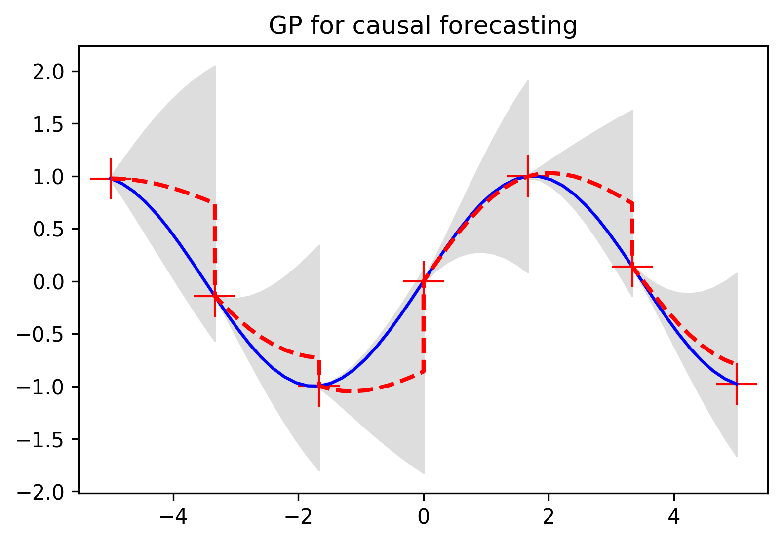
What we see happening in this plot is the Gaussian process using its kernel and available observations to make the same kind of confidence interval predictions that we saw in the interpolation examples, but here we're adding to our observation set as we move along the function domain. Just as you'd imagine, the uncertainty around our prediction shrinks to nothing when we get a new observation, and our mean prediction snaps to the value we just observed. With our updated observation set we then continue calculating confidence intervals, but now benefitting from another point informing our predictions.
When we think of a regression task, we imagine fitting a function to a set of points that someone hands us. However, when you take a step back and think about the nature of what "prediction" is, it seems completely bizarre that we might consider a regression task solved with the output of a single function. Gaussian processes are deeply intuitive objects that let us tell a complete story about the function we're predicting.
In the first example we walked through, we bridged the cognitive divide between multivariate Gaussians and continuously-defined functions by building up a variable component by component until we had a value for every possible point along our domain. Thanks to the ability to calculate marginal distributions of Gaussians, confidence intervals came with each of these infinitely many components. By this point, we realized that what we had defined was just the function equivalent of a Gaussian distribution — where in the single-dimensional case we would draw a sample from a distribution with a mean and variance, here we could draw an entire function from a distribution with a mean function and a covariance function.
Taking a deeper look into how these covariance functions work, we saw that not only do Gaussian processes give us extra information about uncertainty, but they're capable of being designed to anticipate specific types of trends in the function we're hoping to model.
Finally, using what we learned about how a Gaussian process uses a set of observations to draw conclusions about unknown points, we shifted our perspective to the problem of forecasting, in which we're not just trying to fit a function to a set of points, but we're able to iteratively update our predictions as we make new observations.